44 how to show labels in excel chart
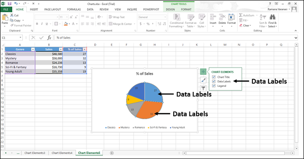
Slope Chart with Data Labels - Peltier Tech In Format all data labels at once on the Mr Excel forum, a user was frustrated with having to format data labels on his slope chart one point at a time, which is a very tedious and frustrating experience.One solution to such tedious tasks is VBA, and I wrote a procedure that would apply and format all data labels at once. The procedure ran instantly, compared to the many minutes it would take ... How to Create Bar of Pie Chart in Excel Tutorial! This will display the values representing each category in the chart. Step 4: To change the display from value to percentage, click on the arrow next to the data labels option. Step 5: Follow the list of options from the dropdown box on the data labels and click on more options. Step 6: you should see the Excel label options in your Excel ...
How to Create and Customize a Treemap Chart in Microsoft Excel Select the data for the chart and head to the Insert tab. Click the "Hierarchy" drop-down arrow and select "Treemap." The chart will immediately display in your spreadsheet. And you can see how the rectangles are grouped within their categories along with how the sizes are determined.

How to show labels in excel chart
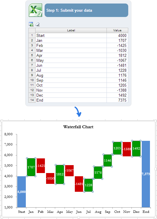
How to Create and Customize a Waterfall Chart in Microsoft ... To fix this, double-click the chart to display the Format sidebar. Select the bar for the total by clicking it twice. Click the Series Options tab in the sidebar and expand Series Options if necessary. Check the box for "Set as Total." Then, do the same for the other total. How to Show Percentage in Pie Chart in Excel? - GeeksforGeeks The steps are as follows : Select the pie chart. Right-click on it. A pop-down menu will appear. Click on the Format Data Labels option. The Format Data Labels dialog box will appear. In this dialog box check the "Percentage" button and uncheck the Value button. This will replace the data labels in pie chart from values to percentage. How to create a progress chart in Excel - spreadsheetweb.com In this guide, we're going to show you how to create a progress chart in Excel. Download Workbook. Steps to create a progress chart 1. Calculate remaining process. Start by calculating the remaining process. If you are using a percentage value, the formula will simply be =1 - <%progress>. 2. Insert a doughnut chart
How to show labels in excel chart. Modifying Axis Scale Labels (Microsoft Excel) - tips Using the Display Units drop-down list, choose Thousands. Click OK. Excel changes the axis values so only the thousands portion is displayed, and inserts a label saying Thousands. Double-click on the Thousands label to edit the label, as desired, then drag it to any desired position. How to create pill charts in Excel - spreadsheetweb.com A pill chart is a fancier way of drawing bar or column charts. Rounded corners and space after axis are enough to make your dashboards catchier. In this guide, we're going to show you How to create pill charts in Excel. Download Workbook[/button. Raw data. The following table is our example dataset. Custom Chart Data Labels In Excel With Formulas Follow the steps below to create the custom data labels. Select the chart label you want to change. In the formula-bar hit = (equals), select the cell reference containing your chart label's data. In this case, the first label is in cell E2. Finally, repeat for all your chart laebls. How To Add Axis Labels In Excel [Step-By-Step Tutorial] First off, you have to click the chart and click the plus (+) icon on the upper-right side. Then, check the tickbox for 'Axis Titles'. If you would only like to add a title/label for one axis (horizontal or vertical), click the right arrow beside 'Axis Titles' and select which axis you would like to add a title/label. Editing the Axis Titles
Prevent Overlapping Data Labels in Excel Charts - Peltier Tech It first loops through the series of the chart, and if the series has a valid label on the point being tested (we text point 1 for the left side labels and point 2 for the right), then the series number and the top position of the label are stored in the array. How to Make a Circle Graph in Excel? | Excel Spy To add data labels, select the pie, right-click, and add data labels. You can see that the dark colors of the slices have made it difficult for the data label fonts to be visible. So, to change the font color of the data labels, select any of the data labels and change the color from the Font Color option. Show/Hide Field Headers in Excel Pivot Tables | MyExcelOnline Whenever you work with Pivot Tables, you can see the Row Labels and Column Labels that are automatically generated on top. This is handy as they can be used to filter out your records.. But, Pivot Table being a tool for the presentation of data as well, you might want to hide these labels as well for making the data set more presentable.It is easy to Show/Hide Field Headers in a Pivot Table. Best Types of Charts in Excel for Data Analysis ... #1 Use a bar chart whenever the axis labels are too long to fit in a column chart: What are the different types of bar charts? Horizontal bar charts - Represent the data horizontally. The data categories are shown on the vertical axis, and data values are shown on the horizontal axis. Vertical bar charts - Also called a column chart.
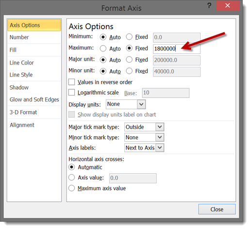
Format Chart Axis in Excel - Axis Options However, In this blog, we will be working with Axis options, Tick marks, Labels, Number > Axis options> Axis options> Format Axis Pane. Axis Options: Axis Options There are multiple options So we will perform one by one. Changing Maximum and Minimum Bounds The first option is to adjust the maximum and minimum bounds for the axis. How can I show percentage change in a clustered bar chart? Double-click it to open the "Format Data Labels" window. Now select "Value From Cells" (see picture below; made on a Mac, but similar on PC). Then point the range to the list of percentages. If you want to have both the value and the percent change in the label, select both Value From Cells and Values. This will create a label like: -12% 1.729.711 How to format bar charts in Excel — storytelling with data More Excel how-to's: To depict a range of values, add a shaded band. To create a frame of reference, embed a vertical line . To show a distribution of data, create a dotplot. For cleaner alignment, put graph elements directly in cells. To have more control over data label formatting, embed labels into your graphs How To Modify A Chart in Microsoft Excel? | Smart Office We just select the drop-down menu and from there we select a predefined Layout for our Chart. Like, for example in the image below the Layout 6 is activated which shows the following Chart Elements: Chart Title, Legend (right) and Percentage Data Label (Best Fit).

How-to Display Metrics Data in an Excel Dashboard Chart - YouTube
Chart.ApplyDataLabels method (Excel) | Microsoft Docs The type of data label to apply. LegendKey: Optional: Variant: True to show the legend key next to the point. The default value is False. AutoText: Optional: Variant: True if the object automatically generates appropriate text based on content. HasLeaderLines: Optional: Variant: For the Chart and Series objects, True if the series has leader ...

How to Create a Pie Chart in Microsoft Excel
A Step-by-Step Guide on How to Make a Graph in Excel After specifying the entries, click on OK. This will display the pie chart on your window. You can click on the icons next to the chart to add your finishing touches to it. Clicking on the chart elements will show you options where you can choose to display or hide data labels, chart tiles, and legend.
How to Show Percentages in Stacked Bar and Column Charts in Excel
How to Show Percentages in Stacked Column Chart in Excel? By default, the data labels are shown in the form of chart data Value (Image 1). But very often user needs to plot charts with actual data and show percentages/custom values on the chart instead of default data. For that we have an option "Value From Cells" in chart "Format Data Label" (Image 2) to select a custom range. Image 1 Image 2

charts - How to change interval between labels in Excel 2013? - Stack Overflow
Display data point labels outside a pie chart in a ... Create a pie chart and display the data labels. Open the Properties pane. On the design surface, click on the pie itself to display the Category properties in the Properties pane. Expand the CustomAttributes node. A list of attributes for the pie chart is displayed. Set the PieLabelStyle property to Outside. Set the PieLineColor property to Black.
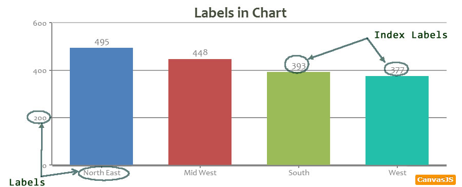
Tutorial on Labels & Index Labels in Chart | CanvasJS JavaScript Charts
How do I add labels to Gantt Chart? - Microsoft Power BI ... You can create a measure like this one that has both values and then use that as your data label. DataLabel = MIN (Sheet1 [Leaving Date]) & " - " & MIN (Sheet1 [Returning Date]) Pat Did I answer your question? Mark my post as a solution! Kudos are also appreciated! To learn more about Power BI, follow me on Twitter or subscribe on YouTube.
Displaying Numbers in Thousands in a Chart in Microsoft Excel | Microsoft Excel Tips from Excel ...
How to Change the Y Axis in Excel - Alphr Click the dropdown next to "Display Units," then make your selection such as "millions" or "hundreds." To label the displayed units, go to the "Axis Options -> Display units" section. Add a...

34 What Is A Category Label In Excel - Labels Design Ideas 2020
How To Create a Burndown Chart in Excel (With Benefits) Related: How To Create a Pivot Tabel in Excel. How to create a burndown chart in Excel. Use the following steps as a general outline for creating a simple burndown chart in Excel: 1. Create a new spreadsheet. Open a new spreadsheet in Excel and create labels for your data. In a simple layout, use the first row for your labels.

Excel chart not printing correctly - i have a simple excel file (office
How to Create a Run Chart in Excel (2021 Guide) | 2 Free ... In the Format Data Series task pane, switch to the Fill & Line tab. Click " Marker. " Select " Marker Options ." In the " Type " dropdown menu, customize your marker type. Set the " Size " value to " 8 ." Add Custom Data Labels You can make your time series plot more informative by adding data labels reflecting the actual values.

Add label to Excel chart line • AuditExcel.co.za
How to Add Labels to Scatterplot Points in Excel - Statology Next, click anywhere on the chart until a green plus (+) sign appears in the top right corner. Then click Data Labels, then click More Options… In the Format Data Labels window that appears on the right of the screen, uncheck the box next to Y Value and check the box next to Value From Cells.
30 Add Label To Excel Chart - Labels Design Ideas 2020
Improve your X Y Scatter Chart with custom data labels Press with right mouse button on on a chart dot and press with left mouse button on on "Add Data Labels" Press with right mouse button on on any dot again and press with left mouse button on "Format Data Labels" A new window appears to the right, deselect X and Y Value. Enable "Value from cells" Select cell range D3:D11
How to Add Labels to an Excel 2007 Chart - Bright Hub
How to Change the X-Axis in Excel - Alphr Follow the instructions to change the text-based X-axis intervals: Open the Excel file and select your graph. Now, right-click on the Horizontal Axis and choose Format Axis… from the menu. Select...
How to create waterfall chart in Excel 2016, 2013, 2010
How To Make The Number Appear On Pie Chart Power Point ... To format data labels, select your chart, and then in the Chart Design tab, click Add Chart Element > Data Labels > More Data Label Options. Click Label Options and under Label Contains, pick the options you want. To make data labels easier to read, you can move them inside the data points or even outside of the chart. How do you label a graph?

34 Label Chart In Excel - Labels Database 2020
How to create a progress chart in Excel - spreadsheetweb.com In this guide, we're going to show you how to create a progress chart in Excel. Download Workbook. Steps to create a progress chart 1. Calculate remaining process. Start by calculating the remaining process. If you are using a percentage value, the formula will simply be =1 - <%progress>. 2. Insert a doughnut chart
35 Label Definition Excel - Labels For Your Ideas
How to Show Percentage in Pie Chart in Excel? - GeeksforGeeks The steps are as follows : Select the pie chart. Right-click on it. A pop-down menu will appear. Click on the Format Data Labels option. The Format Data Labels dialog box will appear. In this dialog box check the "Percentage" button and uncheck the Value button. This will replace the data labels in pie chart from values to percentage.

Teach Besides Me: Data Labels Excel 2010
How to Create and Customize a Waterfall Chart in Microsoft ... To fix this, double-click the chart to display the Format sidebar. Select the bar for the total by clicking it twice. Click the Series Options tab in the sidebar and expand Series Options if necessary. Check the box for "Set as Total." Then, do the same for the other total.
Post a Comment for "44 how to show labels in excel chart"