45 excel pivot table column labels
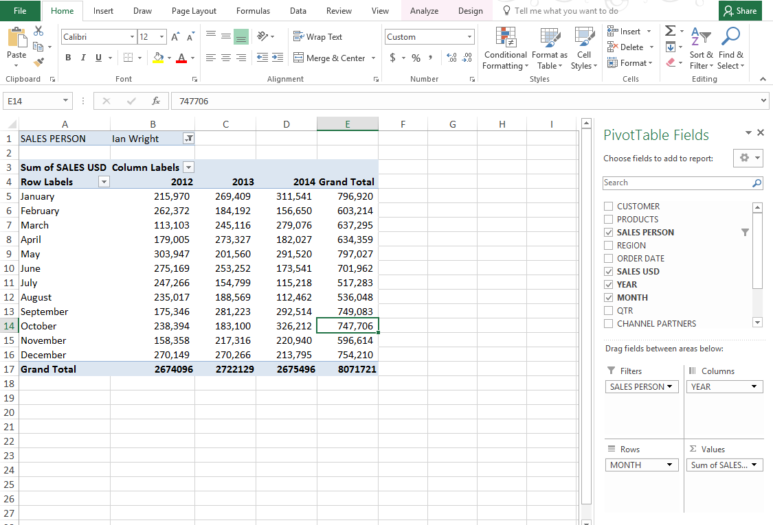
How to Show Percentages in Stacked Column Chart in Excel? Follow the below steps to show percentages in stacked column chart In Excel: Step 1: Open excel and create a data table as below. Step 2: Select the entire data table. Step 3: To create a column chart in excel for your data table. Go to "Insert" >> "Column or Bar Chart" >> Select Stacked Column Chart. Step 4: Add Data labels to the chart. Filter by Labels - Text | MyExcelOnline STEP 1: Click on the Row Label filter button in the Pivot Table. STEP 2: Select Label Filters. You will see that we have a lot of filtering options. Let us try out - Ends With. STEP 3: Type in ber to get the months ending in ber. You can see that the Label Filter will be applied to the SALES MONTH. Click OK.
How to Flatten Data in Excel Pivot Table? - GeeksforGeeks Select a range that you want to flatten - typically, a column of labels. Highlight the empty cells only - hit F5 (GoTo) and select Special > Blanks. Type equals (=) and then the Up Arrow to enter a formula with a direct cell reference to the first data label. Instead of hitting enter, hold down Control and hit Enter.

Excel pivot table column labels
Sorting Row Labels in a Pivot Table by Month - Microsoft Community Sorting Row Labels in a Pivot Table by Month Hoping somebody can help please. I have a Dataset with dates people book holidays. I have a column using the =TEXT (A1,"mmm-yy") to get them grouped by month. I thine put that column in a pivot table but the table doesn't go from January -December. It does it by the first letter so April, Aug, Feb etc., How to Group Columns in Excel Pivot Table (2 Methods) Follow the below steps to create the expected Pivot Table. Steps: First, go to the source data sheet and press Alt + D + P from the keyboard. As a result, the PivotTable and PivotChart Wizard will show up. Click on the Multiple consolidation ranges and PivotTable options as below screenshot and press Next. Column labels multiple contains filters in pivot table The way you have multiple US and Uk in your Regions it makes it seem like each US, UK, "US and UK", "US, UK, EU" are all different countries. You can add Regions Vurrent to either Column filter or or Filter above Next RR Date in your pivot table. hope this helps. 0 Likes.
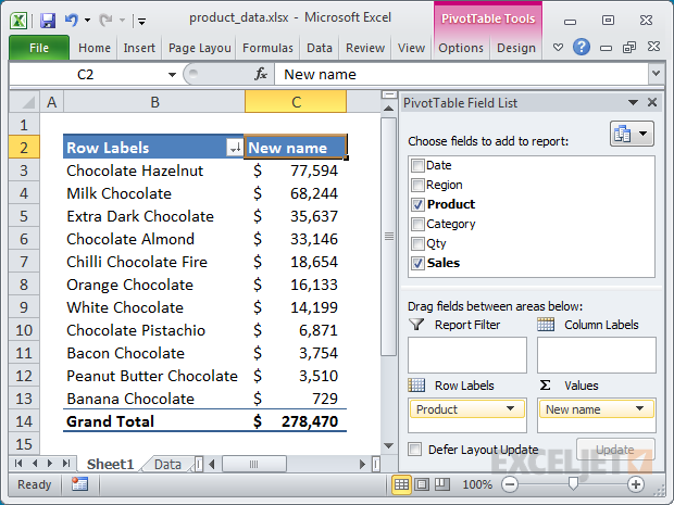
Excel pivot table column labels. Excel Pivot Table Column - Microsoft Tech Community Is there a way to make my own column in a pivot table? I'll provide the existing table for reference: I would like to make a column that simply outputs the difference between "Declined" and "Total" I know I can make a column next to it that easily does this but if the column can somehow exist within the existing table, that will be of great help. Excel filtering pivot table filter/slicer across column label Created on May 15, 2022 Excel filtering pivot table filter/slicer across column label Hello. I have a table with the year as the column headings/labels (2009-2021) and a couple other columns with additional information that aren't a year. The rows represent the specific data for each year. Excel Pivot Table Tutorial - 8bitthis In this Excel pivot table tutorial, we'll learn how to add a calculated field to a Pivot Table report. To add a calculated field, select the Pivot Table report and click the contextual Ribbon tabs. ... Then you can assign grouping labels to each group. After that, you can add the helper column to your pivot table as a column or row field. Excel VBA Macro to Repeat Item Labels in a PivotTable Use the RepeatAllLabels property of the PivotTable object. Options are xlRepeatLabels and xlDoNotRepeatLabels. Dim ws As Worksheet Set ws = ActiveSheet Dim wb As Workbook Set wb = ActiveWorkbook Dim PTcache As PivotCache Dim PT As PivotTable 'Define the cache for the PivotTable Set PTcache =wb.PivotCaches.Create(SourceType:=xlDatabase, _ SourceData:=Range("Sales_Data[#All]"),Version ...
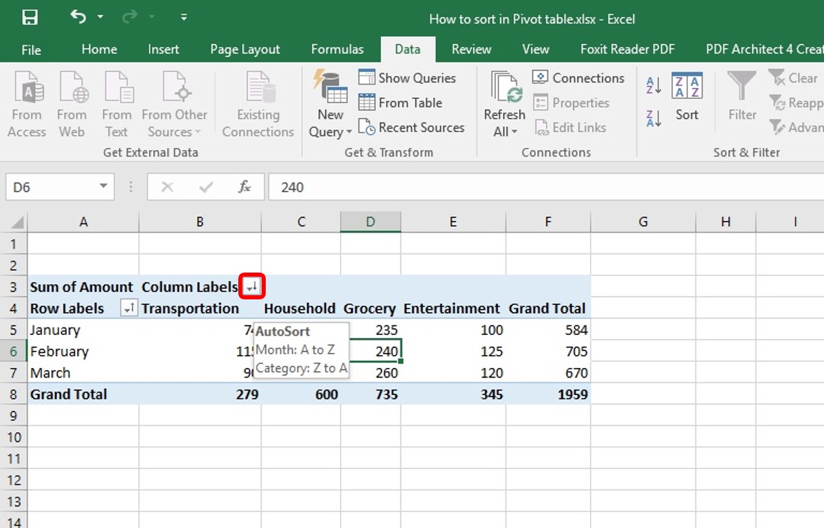
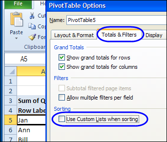
Pivot Table Sorting Trick - Microsoft Tips and Codes - Library Guides ... A quick way to sort columns by a custom list in a pivot table. Once in a while, we have lists that we need to sort in custom ways. The default in a pivot table is alphabetically. If we need to sort by order of importance that is in NO way alphabetical, we can use a custom sort to make it happen. I am going to use a list we use to provide ... Shifting Row Sub label to another column in Pivot Table 37 6. If you are OK with having the country in Column 2, merely change the Report Layout to show in tabular form and you may also want to do not show subtotals. - Ron Rosenfeld. Oct 25, 2021 at 13:44. Add a comment. How to Format Excel Pivot Table - Contextures Excel Tips Follow these steps to create a new pivot table style. First, select a cell in the pivot table Next, on the Excel Ribbon, click the Design tab. In the PivotTable Styles gallery, scroll to the bottom Click the New PivotTable Style command Next, follow the steps in the next section below, to name and modify the new style. Excel Pivot Table Months Or Weekdays Are Alphabetical - 2482 Replies: 2. You have a pivot table in Excel. The months and weekday names are appearing alphabetically instead of in calendar sequence. This happens when your pivot table is based on external data or the data model. There are two solutions. This video prefers using the Custom Sort Order option. This takes 8 clicks to fix the months and 8 clicks ...
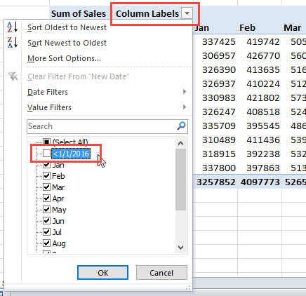
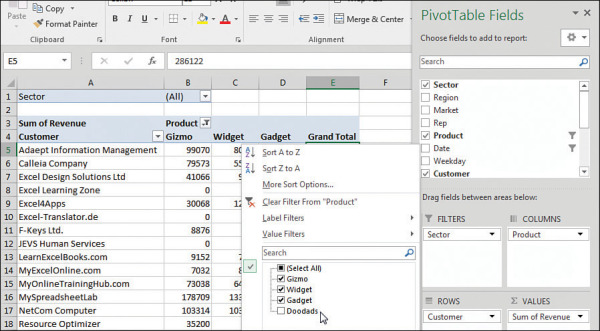
Excel Pivot values as column labels - Stack Overflow If you have Excel for Office 365 (or Excel 2021) with the FILTER function, you can use the following: Note that I used a table with structured references for the data source. This has advantages in editing the table in the future. For "pivot" header: =TRANSPOSE(SORT(UNIQUE(Table1[Country]))) For the columns: How to Use Excel Pivot Table Label Filters - Contextures Excel Tips In an Excel pivot table, you might want to hide one or more of the items in a Row field or Column field. To do that, you could click the drop down arrow for the Row or Column Labels, to see the list of pivot items in that pivot field. Then, in the list, remove the check mark for items you want to remove. Excel: How to Sort Pivot Table by Date - Statology Often you may want to sort the rows in a pivot table in Excel by date. Fortunately this is easy to do using the sorting options in the dropdown menu within the Row Labels column of a pivot table. The following example shows exactly how to do so. Example: Sort Pivot Table by Date in Excel Displaying Row and Column Labels (Microsoft Excel) You specify what rows and columns you want to freeze by selecting the cell immediately below and to the right of the area to be frozen. For instance, if you want to freeze rows 1 through 4 and column A, you would select the cell at B5. Then, to freeze the rows and columns, you select Freeze Panes from the Window menu.
Microsoft Excel – showing field names as headings rather than ...
How To Change Column Names In A Pivot Table | Brokeasshome.com Change Field Names In Pivot Table Source Data Excel Tables. Centre Column Headings In Excel Pivot Table Tables. How To Use Pivot Table Field Settings And Value Setting. Add Multiple Columns To A Pivot Table Custuide. Create A Pivottable Manually. How To Rename Columns In Google Sheets 2 Methods Spreadsheet Point.

Adding a Calculated Item to a Pivot Table in Excel 2010
How To Unpivot Data in Excel (3 Different Ways) | Indeed.com Here are steps to consider for using power query, also known as the get and transform method, to unpivot data in Excel: 1. Put your data into an Excel Table To put your data into a table, click any cell in the dataset and go to the "Insert" tab in the top toolbar. Under the "Tables" section, select "Table." A box appears labeled "Create Table."
Pivot Table Tips | Exceljet
Excel: How to Filter Data in Pivot Table Using "Greater Than" Often you may want to filter values in a pivot table in Excel using a "Greater Than" filter. Fortunately this is easy to do using the Value Filters dropdown menu within the Row Labels column of a pivot table. The following example shows exactly how to do so. Example: Filter Data in Pivot Table Using "Greater Than"
Microsoft Excel Training in Columbus | Make Tech Easy With EasyIT
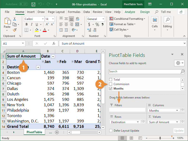
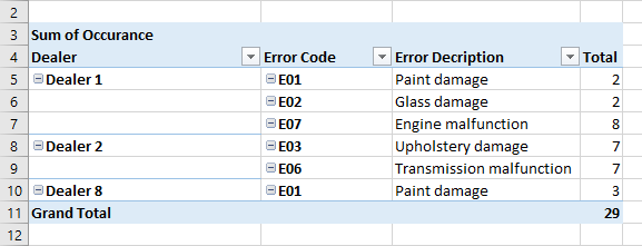
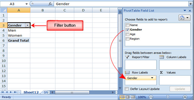
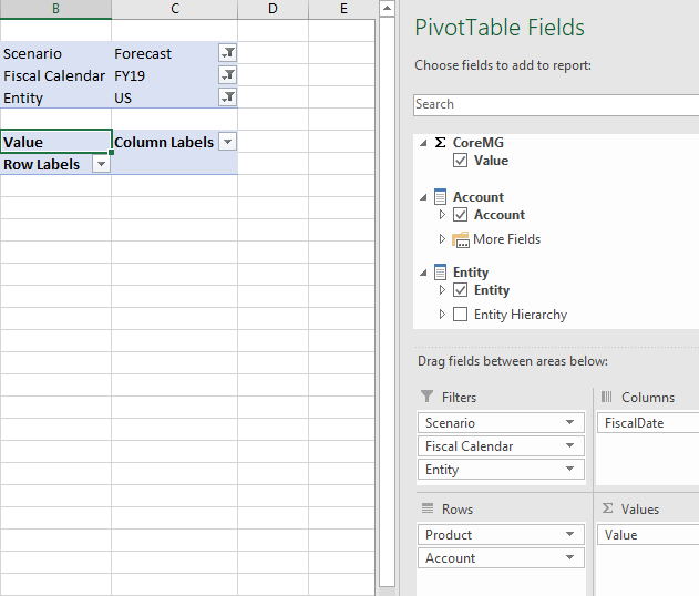
How to make and use Pivot Table in Excel - Ablebits.com When you are creating a Pivot Table, Excel applies the Compact layout by default. This layout displays " Row Labels " and " Column Labels " as the table headings. Agree, these aren't very meaningful headings, especially for novices. An easy way to get rid of these ridiculous headings is to switch from the Compact layout to Outline or Tabular.

Pivot table row labels in separate columns • AuditExcel.co.za
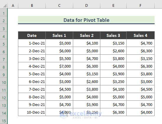
How to Create Excel Pivot Table (Includes practice file) To create an Excel pivot table, Open your original spreadsheet and remove any blank rows or columns. You may also use the Excel sample data at the bottom of this tutorial. Make sure each column has a meaningful label. The column labels will be carried over to the Field List. Verify your columns are properly formatted for their data type.
Pivot Table Filter | CustomGuide
Add filter option for all your columns in a pivot table - Excel Exercise Select the first empty cell after the header column of your pivot table In this situation, the menu Data > Filter is enabled And then, all your pivot table columns have the filter options With all the features related to filters Select a specific values Select larger / smaller than Sort your data Enjoy previous post
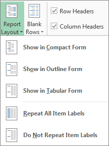
Repeat item labels in a PivotTable
Data Labels in Excel Pivot Chart (Detailed Analysis) 7 Suitable Examples with Data Labels in Excel Pivot Chart Considering All Factors 1. Adding Data Labels in Pivot Chart 2. Set Cell Values as Data Labels 3. Showing Percentages as Data Labels 4. Changing Appearance of Pivot Chart Labels 5. Changing Background of Data Labels 6. Dynamic Pivot Chart Data Labels with Slicers 7.
How To Manage Big Data With Pivot Tables
How to Sort Pivot Table Manually? - Excel Unlocked Click on the button next to Row Labels in cell B3. Click on More Sort Options from there and choose the Manual Sort option. This opens the Sort Dialog box for Pizza Sizes. Choose the first option for Manual Sort. This enables the Manual Sort and now we need to actually manually sort the pivot table rows. Manually Sorting the Data
How to Sort Pivot Table | Custom Sort Pivot Table | A-Z, Z-A ...
Customizing a pivot table | Microsoft Press Store To toggle off those headings, look on the far-right side of the PivotTable Analyze tab for an icon called Field Headers and click it to remove Row Labels and Column Labels from your pivot tables in Compact form. FIGURE 3-19 The Compact form replaces useful headings with Row Labels. You can turn these off. Caution
MS Excel 2013: Display the fields in the Values Section in ...
Calculating Time Between Dates in a Pivot Table For example, if Customer A payment #1 received 1/1/21, payment #2 received 1/11/21, then payment #3 received 1/26/21, then there would be a stacked column chart with a column for Customer A and that column would have two segments, one of value 10 (labeled "payment #2") and the next of value 15 (labeled "payment #3"). Does that make sense?
Filter Pivot Table Columns Labels - Excel Dashboard Templates
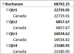
Highlight Cell Rules based on text labels | MyExcelOnline Example 1: This is our current Pivot Table setup. We want to highlight all of the Q1 text in our Row Labels.. STEP 1: Highlight all the quarter text by clicking above the cell STEP 2: Go to Home > Conditional Formatting > Highlight Cells Rules > Text that Contains STEP 3: Type in Q1 and select OK. You can select any color that you wish. The Q1 text is now highlighted!

Removing old Row and Column Items from the Pivot Table ...
Column labels multiple contains filters in pivot table The way you have multiple US and Uk in your Regions it makes it seem like each US, UK, "US and UK", "US, UK, EU" are all different countries. You can add Regions Vurrent to either Column filter or or Filter above Next RR Date in your pivot table. hope this helps. 0 Likes.
Pivot table row labels side by side – Excel Tutorials
How to Group Columns in Excel Pivot Table (2 Methods) Follow the below steps to create the expected Pivot Table. Steps: First, go to the source data sheet and press Alt + D + P from the keyboard. As a result, the PivotTable and PivotChart Wizard will show up. Click on the Multiple consolidation ranges and PivotTable options as below screenshot and press Next.

Creating Pivot Tables in Excel for Exported Data – Teaching ...
Sorting Row Labels in a Pivot Table by Month - Microsoft Community Sorting Row Labels in a Pivot Table by Month Hoping somebody can help please. I have a Dataset with dates people book holidays. I have a column using the =TEXT (A1,"mmm-yy") to get them grouped by month. I thine put that column in a pivot table but the table doesn't go from January -December. It does it by the first letter so April, Aug, Feb etc.,

Excel Pivot Tables: A Comprehensive Guide

Use the Field List to arrange fields in a PivotTable
Centre Column Headings in Excel Pivot Table | Excel Pivot Tables

Automatic Row And Column Pivot Table Labels
Excel Pivot Tables Explained • My Online Training Hub

How to Use Excel Pivot Table Label Filters
Show/Hide Field Headers in Excel Pivot Tables | MyExcelOnline

Pivot table row labels in separate columns • AuditExcel.co.za
Excel Pivot Tables - Sorting Data
Lesson 54: Pivot Table Row Labels - Swotster

Excel Pivot Tables: Insert Calculated Fields & Calculated ...
MS Excel Pivot Table Deleted Items Remain - Excel and Access
Pivot Table Tips | Exceljet
How to Group Columns in Excel Pivot Table (2 Methods) - ExcelDemy

How to Show Hide Field Header In Pivot Table in Excel
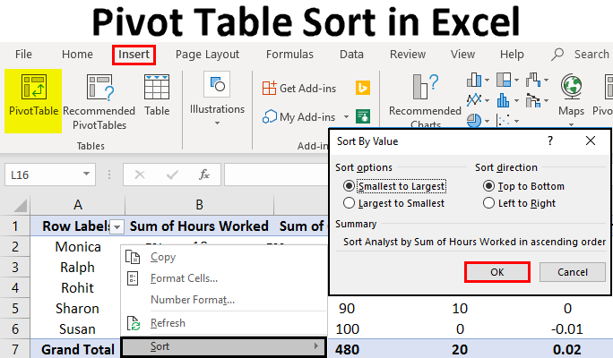
Pivot Table Sort in Excel | How to Sort Pivot Table Columns ...

Pivot table row labels side by side – Excel Tutorials
My Biggest Pivot Table Annoyance (And How To Fix It ...
Why is there no Data in my PivotTable? – Kepion Support Center

How to make row labels on same line in pivot table?
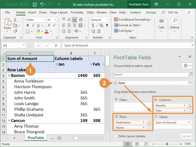
Add Multiple Columns to a Pivot Table | CustomGuide
Excel Pivot Table Sorting Problems – Contextures Blog
Automatic Row And Column Pivot Table Labels
Excel Pivot table: Change the Number format of Column label ...
Design the layout and format of a PivotTable
Instructions for Sorting a Pivot Table by Two Columns | Excelchat

How to make row labels on same line in pivot table?

VBA to grab Pivot Table Column Names | MrExcel Message Board
Grouping, sorting, and filtering pivot data | Microsoft Press ...

Excel Pivot Tables: A Comprehensive Guide

How to use another column as X axis label when you plot pivot ...
Post a Comment for "45 excel pivot table column labels"